
Monte Carlo simulation is a powerful mathematical technique that can be used to model a wide range of systems, from financial markets to physical systems. At its core, Monte Carlo simulation is based on the idea of using random sampling to understand the underlying probability distributions of a system.
The basic idea behind Monte Carlo simulation is simple: imagine you have a coin and you want to know the probability of getting heads or tails. One way to do this would be to flip the coin a large number of times and keep track of the number of heads and tails. As you flip the coin more and more times, the ratio of heads to tails will converge towards the true probability of getting heads or tails – 50/50.
This is the fundamental principle behind Monte Carlo simulation: by repeatedly running a simulation and randomly sampling from the underlying probability distributions, we can gain a better understanding of the system as a whole.
Similarly, in the case of cyber risks, we can use Monte Carlo simulation to estimate the total cyber-value-at-risk for a portfolio of cyber threats by running many simulations, each time randomly sampling from the probability distributions of the different cyber threats.
The script first defines a Pandas DataFrame with the cyber events, probability of occurrence and the impact in dollars in a upper and lower range. It then defines four functions:
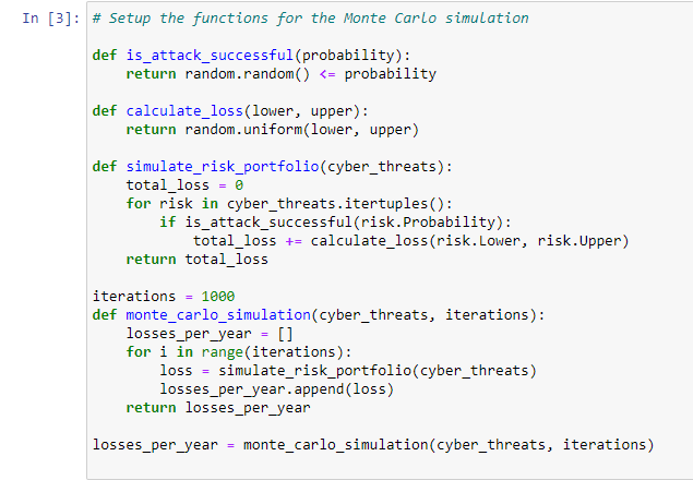
is_attack_successful(probability): This function generates a random number between 0 and 1 and compares it to the probability of an attack passed as an argument. If the random number is less than or equal to the probability, the function returns True, indicating a successful attack. If not, it returns False.
calculate_loss(lower, upper): This function generates a random number between the lower and upper bounds of loss passed as arguments and returns it.
simulate_risk_portfolio(cyber_threats): This function loops through each risk in the cyber_threats DataFrame and uses the is_attack_successful function to determine if the attack is successful. If it is, it calculates the loss using the calculate_loss function and adds it to the total loss. The function then returns the total loss.
monte_carlo_simulation(cyber_threats, iterations): This function runs the simulation by calling the simulate_risk_portfolio function for a specified number of iterations passed as an argument. It stores the result of each iteration in the losses_per_year list and returns it.
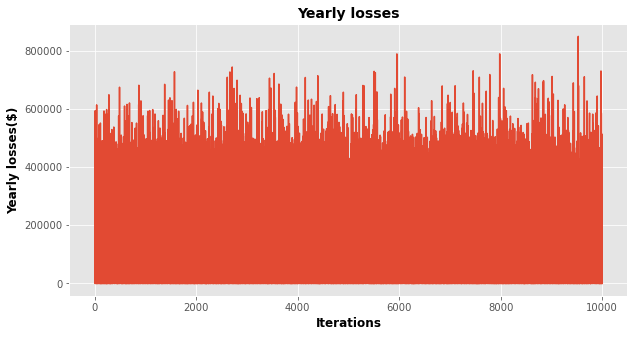
We can then plot the losses per year as well as the loss-exceedance curve:
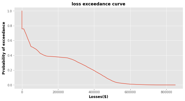
A loss-exceedance curve is a graph that shows the likelihood of different loss amounts occurring. It is often used in the field of risk management to help understand the potential losses from a specific event, such as a natural disaster or cyber attack. The x-axis of the graph shows the different loss amounts and the y-axis shows the probability of that loss happening. The curve is usually plotted from the highest loss amount to the lowest, with the highest loss amount having the lowest probability of happening and the lowest loss amount having the highest probability of happening. This type of graph helps to understand the potential risks and allows for more informed decision making.
An additional topic that is worth mentioning is convergence. In the context of a Monte Carlo simulation, it refers to the point at which the output of the simulation becomes stable and consistent, regardless of the number of iterations run. In other words, the simulation results no longer change significantly with an increase in the number of iterations. This is important because it means that the simulation has run enough iterations to accurately represent the underlying system being modeled. In the case of a cyber-risk simulation, convergence means that the annualized losses become consistent, regardless of the number of iterations run.
The Python Jupyter notebook with the code for this Monte Carlo simulation can be found here and it additionally contains descriptive statistics and the annualised loss for the different cyber threats – this can be really helpful in the comparison of different scenarios, or for forecasting future losses.
However, this is a simplified example. There are several ways it can be improved and built upon. Consider including:
- Confidence Interval: You could use the results of the simulation to calculate a confidence interval for the expected losses. This would give you an idea of the range of possible losses given the simulated results.
- Sensitivity Analysis: You could run the simulation multiple times, each time changing one of the parameters (e.g. probability of attack, lower bound of loss, upper bound of loss) to see how the results change. This would give you an idea of which parameters have the biggest impact on the results.
- Compare the results with industry standards: you could compare the results of the simulation with industry standards in terms of the frequency and severity of losses, this would allow you to evaluate the realism of the simulation and adjust it accordingly.
- Additional Mitigation Scenarios: you could add more mitigation scenarios, such as different types of controls or different levels of investment, and compare the results to see which scenario is the most cost-effective.
Overall, this script provides a powerful tool for understanding and quantifying the cyber risks in a portfolio. By using a Monte Carlo simulation, we can generate a large number of potential outcomes, giving us a more comprehensive understanding of the risks and the potential impact.
Leave a Reply